Basic inverse kinematics in MuJoCo

In my journey exploring the fundamentals of robot manipulation, I was curious about how to perform simple inverse kinematics. I'm aware that numerous libraries exist to handle this topic, but I'd like to practice translating the math/pseudocode into actual implementation, particularly in MuJoCo, which is my primary simulator for conducting experiments at the moment. Here's what I discovered:

What is inverse kinematics

Imagine you have a six-joint robot manipulator with an end-effector, like a gripper, at its tip. You want to move this end-effector to a specific point in 3D space to perform a task. To achieve this, you need to determine the exact joint coordinates required to position the end-effector at your desired point. This is where inverse kinematics comes into play.

Inverse kinematics is the process of mapping the end-effector's pose (position and orientation) to the joint coordinates that will achieve that pose. By using inverse kinematics, you can find the specific joint angles needed to move the end-effector to your desired point in 3D space.

ik-diagram

Given that there are two ways to solve inverse kinematics: the analytical approach and the numerical approach. The analytical approach involves using the mathematical model to solve for the joint angles required to achieve a desired end-effector pose. On the other hand, the numerical approach involves using iterative calculations to approximate the joint angles using an optimization algorithm.

In this article I will focus on the numerical approaches that I found.

Inverse Kinematics algorithms

While searching for the most common ways to compute inverse kinematics, I discovered the master thesis of Anton Larsson and Oskar Grönlund titled "Comparative Analysis of the Inverse Kinematics of a 6-DOF Manipulator". In this thesis, they discuss the use of the Jacobian to approximate the relationship between joint angles and desired end-effector position. They explain three methods for doing this: Gradient Descent, Gauss-Newton, and Levenberg-Marquardt.

Gauss-Newton

The Gauss-Newton algorithm is a extension of a Newton's method for finding a minimum value of a non-linear function [1]. It starts by defining an initial guess $x_{n}$ and estimate the next best optimal value denote by $x_{n+1}$ using the equation (1).

\begin{align} x_{n+1} = x_{n} - \frac{f^{\prime}(x_{n})}{f^{\prime\prime}(x_{n})} \end{align}

Where $f^{\prime}(x_{n})$ represents the gradient of the cost function at the current point $x_{n}$ , while $f^{\prime\prime}(x_{n})$ denotes the second derivative of the cost function at the same point, known as the "Hessian matrix". The Hessian matrix measures how the gradient changes as the parameters change. This equation updates the current point $x_{n}$ by moving in a direction that minimizes the cost function, considering both the gradient and the curvature of the cost function at that point. If you'd like to explore this technique further, I recommend referring to the thesis by Anton and Oskar for more detailed information.

The Gauss-Newton method approximates the Hessian matrix using the Jacobian matrix to establish the relationship between joints and end-effector position. However, in Anton and Oskar's thesis, they utilize the pseudo-inverse of the Jacobian matrix, as seen in equation (2), instead of the original version.

\begin{align} J^{\dagger} = (J^{T}J)^{-1}J^{T} \end{align}

Then the equation (1) turns to.

\begin{align} x_{n+1} = x_{n} - H^{-1}\nabla f(x_{n}) = x_{n} - J^{\dagger}r(x) \end{align}

In the thesis, they also provides a pseudocode to use.

goal_pose = y
q = current joint angles
step_size = desired step size
tolerance = set tolerance
e = goal_pose - current_pose
while norm(e) >= tolerance do
    J = Jacobian(q)
    J_T = J.transpose()
    J_pinv = (J_T * J).inv() * J_T
    delta_q = J_pinv * e
    q += step_size * delta_q
    q = check_joint_limits(q)
    e = goal_pose - ForwardKinematics(q)
end while

Gradient Descent

The gradient descent method, also known as the Jacobian transpose method, is another numerical approach to solving the inverse kinematics optimization problem. This method solves the problem by iteratively adjusting the joint angles to reduce the error between the desired and actual end-effector position.

In order to obtain the joint angles, the gradient descent method utilizes the transpose of the Jacobian matrix to map the difference between the actual and desired end-effector positions to the angles of the joints [2]. This is achieved by calculating the gradient using equation (3)

\begin{align} x_{n+1} = x_{x} - \alpha \nabla f(x_{n}) = x_{n} - \alpha J^{T}r(x) \end{align}

Where $\alpha$ is the learning rate that define the size of the step taken into the direction of the steepest descent during each iteraction [2]. Also is commun to define this parameter by trial and error.

goal_pose = y
q = current joint angles
step_size = desired step size
tolerance = set tolerance
e = goal_pose - current_pose
while norm(e) >= tolerance do
    J = Jacobian(q)
    J_T = J.transpose()
    gradient = alpha * J_T * e
    q += step_size * gradient
    q = check_joint_limits(q)
    e = goal_pose - ForwardKinematics(q)
end while

Levenberg-Marquardt

The Levenberg-Marquardt method, is a combination of Gauss-Newton and gradient descent using the following equation.

\begin{align} x_{n+1} = x_{n} + (J^{T}J + \lambda I)^{-1}J^{T}r(x_{n}) \end{align}

Where $x_{n}$ represents the current value of x at the n-th iteration, $J$ is the Jacobian matrix of the $f(x)$ function, $r(x_{n})$ denotes the residual vector at $x_{n}$ , $\lambda$ is a damping factor used to control the step size, and $I$ represents the identity matrix.

Similar to $\alpha$ , the parameter $\lambda$ is also determined through a process of trial and error.

goal_pose = y
q = current joint angles
step_size = desired step size
tolerance = set tolerance
e = goal_pose - current_pose
lambda = damping factor

while norm(e) >= tolerance do
    J = Jacobian(q)
    J_T = Jacobian.transpose()
    J_inv = (J_T * J + lambda * I).inv() * J_T
    delta_q = J_inv * e
    q += step_size * delta_q
    q = check_joint_limits(q)
    e = goal_pose - ForwardKinematics(q)
end while

Implementation

Seeing that they provide the pseudocode for each algorithm, I have the idea of trying to re-implement these techniques in MuJoCo for practice. Let me explain how I do it.

First, you need to install the necessary libraries for coding. In this case, I decided to use the Python bindings of the MuJoCo library.

import numpy as np
import mujoco
import mujoco.viewer as viewer
import mediapy as media

Then, choose a MuJoCo robot arm model to test our inverse kinematics. In this case I decided to use the UR5e robot arm from the mujoco_menangerie library

#add path
xml = "<path>/mujoco_menagerie/universal_robots_ur5e/scene.xml"
model = mujoco.MjModel.from_xml_path(xml)
data = mujoco.MjData(model)
renderer = mujoco.Renderer(model)

I also created a new camera, to get a better view of the robot.

camera = mujoco.MjvCamera()
mujoco.mjv_defaultFreeCamera(model, camera)
camera.distance = 1

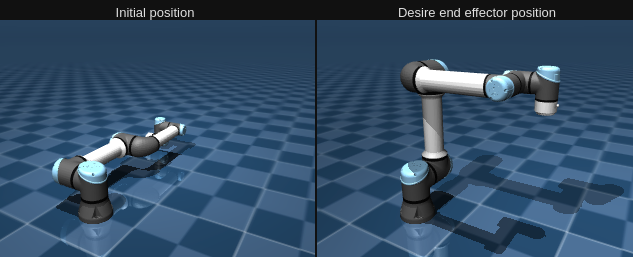
One important thing to ensure the correctness of an algorithm is to have a "test coordinate." To do this, I choosed the position of the joints that give a good visualization by trial and error and use the "wrist 3" link, which is the last piece of the robot model, as an end-effector

#Put a position of the joints to get a test point
pi = np.pi
data.qpos = [3*pi/2, -pi/2, pi/2, 3*pi/2, 3*pi/2, 0]

#Initial joint position
qpos0 = data.qpos.copy()

#Step the simulation.
mujoco.mj_forward(model, data)

#Use the last piece as an "end effector" to get a test point in cartesian 
# coordinates
target = data.body('wrist_3_link').xpos
print("Target =>",target)

#Plot results
print("Results")
mujoco.mj_resetDataKeyframe(model, data, 1)
mujoco.mj_forward(model, data)
init_point = data.body('wrist_3_link').xpos.copy()
renderer.update_scene(data, camera)
target_plot = renderer.render()

data.qpos = qpos0
mujoco.mj_forward(model, data)
result_point = data.body('wrist_3_link').xpos.copy()
renderer.update_scene(data, camera)
result_plot = renderer.render()

print("initial point =>", init_point)
print("Desire point =>", result_point, "\n")

images = {
    'Initial position': target_plot,
    ' Desire end effector position': result_plot,
}

media.show_images(images)

And this is what I've got.

test coordinate

Now let's create the algorithms.

As you can see in the pseudocode, there is something similar among all of them, which is that they all use the Jacobian. Fortunately, MuJoCo provides a method that allows us to calculate the Jacobian without having to do it manually, which is called mj_jac. It can be a big help in creating these algorithms.

I created a class for the different algorithms to make their use simpler. In this class, I defined the check_joint_limits method in the pseudocode and the calculate method, where I implemented the algorithm using the MuJoCo library and NumPy.

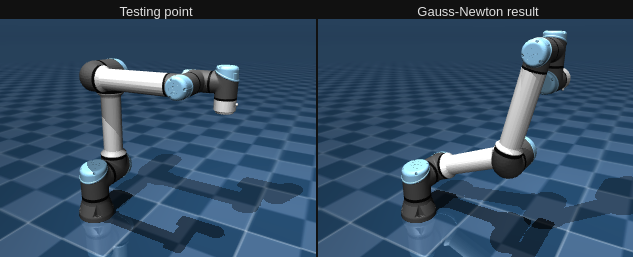
After implementing the algorithms, I initialized the variables for each one. These values change a lot depending on the distance from the starting angles, so I determined the values through the results of Anton&Oskar thesis and trial and error to find what works best. However, if you want to experiment with the parameters, feel free to do so. Finally, I rendered the model and checked if it works.

Gradient descent

# Gradient Descent method
class GradientDescentIK:
    
    def __init__(self, model, data, step_size, tol, alpha, jacp, jacr):
        self.model = model
        self.data = data
        self.step_size = step_size
        self.tol = tol
        self.alpha = alpha
        self.jacp = jacp
        self.jacr = jacr
    
    def check_joint_limits(self, q):
        """Check if the joints is under or above its limits"""
        for i in range(len(q)):
            q[i] = max(self.model.jnt_range[i][0], 
                       min(q[i], self.model.jnt_range[i][1]))

    #Gradient Descent pseudocode implementation
    def calculate(self, goal, init_q, body_id):
        """Calculate the desire joints angles for goal"""
        self.data.qpos = init_q
        mujoco.mj_forward(self.model, self.data)
        current_pose = self.data.body(body_id).xpos
        error = np.subtract(goal, current_pose)

        while (np.linalg.norm(error) >= self.tol):
            #calculate jacobian
            mujoco.mj_jac(self.model, self.data, self.jacp, 
                          self.jacr, goal, body_id)
            #calculate gradient
            grad = self.alpha * self.jacp.T @ error
            #compute next step
            self.data.qpos += self.step_size * grad
            #check joint limits
            self.check_joint_limits(self.data.qpos)
            #compute forward kinematics
            mujoco.mj_forward(self.model, self.data) 
            #calculate new error
            error = np.subtract(goal, self.data.body(body_id).xpos)

#Init variables.
body_id = model.body('wrist_3_link').id
jacp = np.zeros((3, model.nv)) #translation jacobian
jacr = np.zeros((3, model.nv)) #rotational jacobian
goal = [0.49, 0.13, 0.59]
step_size = 0.5
tol = 0.01
alpha = 0.5
init_q = [0.0, 0.0, 0.0, 0.0, 0.0, 0.0]

ik = GradientDescentIK(model, data, step_size, tol, alpha, jacp, jacr)

#Get desire point
mujoco.mj_resetDataKeyframe(model, data, 1) #reset qpos to initial value
ik.calculate(goal, init_q, body_id) #calculate the q angles

result = data.qpos.copy()

#Plot results
print("Results")
data.qpos = qpos0
mujoco.mj_forward(model, data)
renderer.update_scene(data, camera)
target_plot = renderer.render()

data.qpos = result
mujoco.mj_forward(model, data)
result_point = data.body('wrist_3_link').xpos
renderer.update_scene(data, camera)
result_plot = renderer.render()

print("testing point =>", target)
print("Gradient Descent result =>", result_point, "\n")

images = {
    'Testing point': target_plot,
    'Gradient Descent result': result_plot,
}

media.show_images(images)

gd-result-render

Gauss-Newton

# Gauss-Newton method
class GaussNewtonIK:
    
    def __init__(self, model, data, step_size, tol, alpha, jacp, jacr):
        self.model = model
        self.data = data
        self.step_size = step_size
        self.tol = tol
        self.alpha = alpha
        self.jacp = jacp
        self.jacr = jacr
    
    def check_joint_limits(self, q):
        """Check if the joints is under or above its limits"""
        for i in range(len(q)):
            q[i] = max(self.model.jnt_range[i][0], 
                       min(q[i], self.model.jnt_range[i][1]))
    
    # Gauss-Newton pseudocode implementation
    def calculate(self, goal, init_q, body_id):
        """Calculate the desire joints angles for goal"""
        self.data.qpos = init_q
        mujoco.mj_forward(self.model, self.data)
        current_pose = self.data.body(body_id).xpos
        error = np.subtract(goal, current_pose)

        while (np.linalg.norm(error) >= self.tol):
            #calculate jacobian
            mujoco.mj_jac(self.model, self.data, self.jacp, 
                          self.jacr, goal, body_id)
            #calculate delta of joint q
            product = self.jacp.T @ self.jacp
            
            if np.isclose(np.linalg.det(product), 0):
                j_inv = np.linalg.pinv(product) @ self.jacp.T
            else:
                j_inv = np.linalg.inv(product) @ self.jacp.T
            
            delta_q = j_inv @ error
            #compute next step
            self.data.qpos += self.step_size * delta_q
            #check limits
            self.check_joint_limits(self.data.qpos)
            #compute forward kinematics
            mujoco.mj_forward(self.model, self.data) 
            #calculate new error
            error = np.subtract(goal, self.data.body(body_id).xpos)


#Init variables.
body_id = model.body('wrist_3_link').id
jacp = np.zeros((3, model.nv)) #translation jacobian
jacr = np.zeros((3, model.nv)) #rotational jacobian
goal = [0.49, 0.13, 0.59]
step_size = 0.5
tol = 0.01
alpha = 0.5
init_q = [0.0, 0.0, 0.0, 0.0, 0.0, 0.0]

ik = GaussNewtonIK(model, data, step_size, tol, alpha, jacp, jacr)

#Get desire point
mujoco.mj_resetDataKeyframe(model, data, 1) #reset qpos to initial value
ik.calculate(goal, init_q, body_id) #calculate the qpos

result = data.qpos.copy()

#Plot results
print("Results")
data.qpos = qpos0
mujoco.mj_forward(model, data)
renderer.update_scene(data, camera)
target_plot = renderer.render()

data.qpos = result
mujoco.mj_forward(model, data)
result_point = data.body('wrist_3_link').xpos
renderer.update_scene(data, camera)
result_plot = renderer.render()

print("testing point =>", target)
print("Gauss-Newton result =>", result_point, "\n")

images = {
    'Testing point': target_plot,
    'Gauss-Newton result': result_plot,
}

media.show_images(images)

gn-result-render

Levenberg-Marquardt

#Levenberg-Marquardt method
class LevenbegMarquardtIK:
    
    def __init__(self, model, data, step_size, tol, alpha, jacp, jacr, damping):
        self.model = model
        self.data = data
        self.step_size = step_size
        self.tol = tol
        self.alpha = alpha
        self.jacp = jacp
        self.jacr = jacr
        self.damping = damping
    
    def check_joint_limits(self, q):
        """Check if the joints is under or above its limits"""
        for i in range(len(q)):
            q[i] = max(self.model.jnt_range[i][0], 
                       min(q[i], self.model.jnt_range[i][1]))

    #Levenberg-Marquardt pseudocode implementation
    def calculate(self, goal, init_q, body_id):
        """Calculate the desire joints angles for goal"""
        self.data.qpos = init_q
        mujoco.mj_forward(self.model, self.data)
        current_pose = self.data.body(body_id).xpos
        error = np.subtract(goal, current_pose)

        while (np.linalg.norm(error) >= self.tol):
            #calculate jacobian
            mujoco.mj_jac(self.model, self.data, self.jacp, self.jacr, goal, body_id)
            #calculate delta of joint q
            n = self.jacp.shape[1]
            I = np.identity(n)
            product = self.jacp.T @ self.jacp + self.damping * I
            
            if np.isclose(np.linalg.det(product), 0):
                j_inv = np.linalg.pinv(product) @ self.jacp.T
            else:
                j_inv = np.linalg.inv(product) @ self.jacp.T
            
            delta_q = j_inv @ error
            #compute next step
            self.data.qpos += self.step_size * delta_q
            #check limits
            self.check_joint_limits(self.data.qpos)
            #compute forward kinematics
            mujoco.mj_forward(self.model, self.data) 
            #calculate new error
            error = np.subtract(goal, self.data.body(body_id).xpos)

#Init variables.
body_id = model.body('wrist_3_link').id
jacp = np.zeros((3, model.nv)) #translation jacobian
jacr = np.zeros((3, model.nv)) #rotational jacobian
goal = [0.49, 0.13, 0.59]
step_size = 0.5
tol = 0.01
alpha = 0.5
init_q = [0.0, 0.0, 0.0, 0.0, 0.0, 0.0]
damping = 0.15

ik = LevenbegMarquardtIK(model, data, step_size, tol, alpha, jacp, jacr, damping)

#Get desire point
mujoco.mj_resetDataKeyframe(model, data, 1) #reset qpos to initial value
ik.calculate(goal, init_q, body_id) #calculate the qpos

result = data.qpos.copy()

#Plot results
print("Results")
data.qpos = qpos0
mujoco.mj_forward(model, data)
renderer.update_scene(data, camera)
target_plot = renderer.render()

data.qpos = result
mujoco.mj_forward(model, data)
result_point = data.body('wrist_3_link').xpos
renderer.update_scene(data, camera)
result_plot = renderer.render()

print("testing point =>", target)
print("Levenberg-Marquardt result =>", result_point, "\n")

images = {
    'Testing point': target_plot,
    'Levenberg-Marquardt result': result_plot,
}

media.show_images(images)

lk-result-render

Simulation

Let's try to simulate this movement. To understand how to implement it, I based on the mjctrl repository from Kevin Zakka, where he explains clear and pedagogical implementations of robotics controllers, and by referencing the Mujoco colab examples to render the simulations.

I implemented this code in a Jupyter notebook, and to visualize my robot, I render a video of it. First, I set up the video parameters so that the video can run for 4 seconds.

#Video setup
import mediapy as media

DURATION = 4 #(seconds)
FRAMERATE = 60 #(Hz)
frames = []

Then, I reset the model data, initialize the parameters, and obtain the initial error for the simulation. In this case, I used the Levenberg-Marquardt method.

#Reset state and time
mujoco.mj_resetData(model, data)

#Init parameters
jacp = np.zeros((3, model.nv)) #translation jacobian
jacr = np.zeros((3, model.nv)) #rotational jacobian
step_size = 0.5
tol = 0.01
alpha = 0.5
damping = 0.15

#Get error.
end_effector_id = model.body('wrist_3_link').id #"End-effector we wish to control.
current_pose = data.body(end_effector_id).xpos #Current pose

goal = [0.49, 0.13, 0.59] #Desire position

error = np.subtract(goal, current_pose) #Init Error

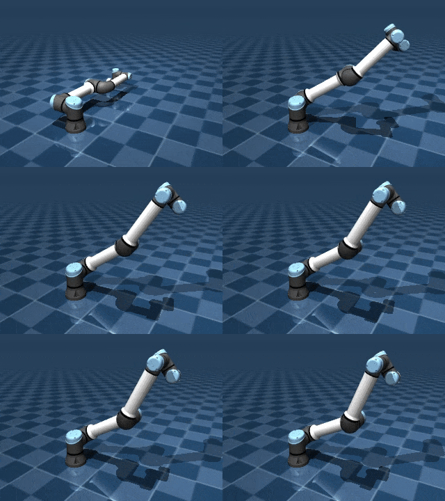
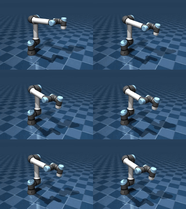
I implemented the algorithm into a loop during the "DURATION" of the video, calculating and updating inverse kinematics on each step frame. The difference between this simulation and the last class implementations is the mj_step method, which integrates in time and advances the simulation, applying forward kinematics. Finally, I rendered and saved frames and displayed them using the MediaPy library.

#Simulate
while data.time < DURATION:
       
    if (np.linalg.norm(error) >= tol):
        #Calculate jacobian
        mujoco.mj_jac(model, data, jacp, jacr, goal, end_effector_id)
        #Calculate delta of joint q
        n = jacp.shape[1]
        I = np.identity(n)
        product = jacp.T @ jacp + damping * I

        if np.isclose(np.linalg.det(product), 0):
            j_inv = np.linalg.pinv(product) @ jacp.T
        else:
            j_inv = np.linalg.inv(product) @ jacp.T

        delta_q = j_inv @ error

        #Compute next step
        q = data.qpos.copy()
        q += step_size * delta_q
        
        #Check limits
        check_joint_limits(data.qpos)
        
        #Set control signal
        data.ctrl = q
        #Step the simulation.
        mujoco.mj_step(model, data)

        error = np.subtract(goal, data.body(end_effector_id).xpos)
    
    #Render and save frames.
    if len(frames) < data.time * FRAMERATE:
        renderer.update_scene(data)
        pixels = renderer.render()
        frames.append(pixels)
        
#Display video.
media.show_video(frames, fps=FRAMERATE)

And this was the final result.

robot

From here you can implement a lot of stuff, like creating a circle similar to mjctrl examples.

robot circle

Here is a full code implementation.

import numpy as np
import mujoco
import mujoco.viewer as viewer
import mediapy as media

#Video Setup
DURATION = 4 #(seconds)
FRAMERATE = 60 #(Hz)
frames = []

#Reset state and time.
mujoco.mj_resetData(model, data)

#Init position.
# pi = np.pi
# data.qpos = [3*pi/2, -pi/2, pi/2, 3*pi/2, 3*pi/2, 0] #ENABLE if you want test circle

#Init parameters
jacp = np.zeros((3, model.nv)) #translation jacobian
jacr = np.zeros((3, model.nv)) #rotational jacobian
step_size = 0.5
tol = 0.01
alpha = 0.5
damping = 0.15

#Get error.
end_effector_id = model.body('wrist_3_link').id #"End-effector we wish to control.
current_pose = data.body(end_effector_id).xpos #Current pose

goal = [0.49, 0.13, 0.59] #Desire position

error = np.subtract(goal, current_pose) #Init Error

def check_joint_limits(q):
    """Check if the joints is under or above its limits"""
    for i in range(len(q)):
        q[i] = max(model.jnt_range[i][0], min(q[i], model.jnt_range[i][1]))

def circle(t: float, r: float, h: float, k: float, f: float) -> np.ndarray:
    """Return the (x, y) coordinates of a circle with radius r centered at (h, k)
    as a function of time t and frequency f."""
    x = r * np.cos(2 * np.pi * f * t) + h
    y = r * np.sin(2 * np.pi * f * t) + k
    z = 0.5
    return np.array([x, y, z])

#Simulate
while data.time < DURATION:
    
    # goal = circle(data.time, 0.1, 0.5, 0.0, 0.5) #ENABLE to test circle.
    
    if (np.linalg.norm(error) >= tol):
        #Calculate jacobian
        mujoco.mj_jac(model, data, jacp, jacr, goal, end_effector_id)
        #Calculate delta of joint q
        n = jacp.shape[1]
        I = np.identity(n)
        product = jacp.T @ jacp + damping * I

        if np.isclose(np.linalg.det(product), 0):
            j_inv = np.linalg.pinv(product) @ jacp.T
        else:
            j_inv = np.linalg.inv(product) @ jacp.T

        delta_q = j_inv @ error

        #Compute next step
        q = data.qpos.copy()
        q += step_size * delta_q
        
        #Check limits
        check_joint_limits(data.qpos)
        
        #Set control signal
        data.ctrl = q 
        #Step the simulation.
        mujoco.mj_step(model, data)

        error = np.subtract(goal, data.body(end_effector_id).xpos)
    
    #Render and save frames.
    if len(frames) < data.time * FRAMERATE:
        renderer.update_scene(data)
        pixels = renderer.render()
        frames.append(pixels)
        
#Display video.
media.show_video(frames, fps=FRAMERATE)

Conclusion

So that's all for now! You've seen how MuJoCo can be used to implement simple Inverse Kinematics. Keep in mind that this approach may not always produce optimal values for your specific needs and may not consider orientation. From here, you can start experimenting with different techniques to fine-tune your implementations using the libraries that I used.

If you find any errors or would like to add more information, please DM me on Twitter/x or send me an email to update this post. I would appreciate it.

You can check the full Jupyter notebook here

I hope this has been helpful, and don't forget to share it with anyone who needs it.

Reference

[1] Gauss–Newton algorithm wikipedia
[2] Anton Larsson and Oskar Grönlund Comparative Analysis of the Inverse Kinematics of a 6-DOF Manipulator
[3] Levenberg-Marquardt algorithm wikipedia
[4] MuJoCo Python Bindings docs Docs
[5] mujoco_menagerie UR5e
[6] kevinzakka mjctrl repo
[7] Deepmind mujoco repo